Regression on Mauna Loa data¶

This example does regression on the Hawaiian Mauna Loa data (example taken from chapter $5$ of the GPML book by Rasmussen and Williams, 2006)

We will use a modelling problem concerning the concentration of $CO_2$ in the atmosphere to illustrate how the marginal likelihood can be used to set multiple hyperparameters in hierarchical Gaussian process models. A complex covariance function is derived by combining several different kinds of simple covariance functions, and the resulting model provides an excellent fit to the data as well as insight into its properties by interpretation of the adapted hyperparameters. Although the data is one-dimensional, and therefore easy to visualize, a total of $11$ hyperparameters are used, which in practice rules out the use of cross-validation for setting parameters, except for the gradient-based LOO-CV procedure.

The data [1] consists of monthly average atmospheric $CO_2$ concentrations (in parts per million by volume (ppmv)) derived from in-situ air samples collected at the Mauna Loa Observatory, Hawaii, between $1958$ and $2003$ (with some missing values) [2].

The data is shown in the above plot. Our goal is to model the $CO_2$ concentration as a function of time $t$ . Several features are immediately apparent: a long term rising trend, a pronounced seasonal variation and some smaller irregularities. In the following, contributions to a combined covariance function which takes care of these individual properties are suggessted. This is meant primarily to illustrate the power and flexibility of the Gaussian process framework—it is possible that other choices would be more appropriate for this data set.

To model the long term smooth rising trend, a squared exponential (SE) covariance term with two hyperparameters controlling the amplitude $\theta_1$ and characteristic length-scale $\theta_2$ is used:

$k_1(x,x') = \theta_1^2 \exp \left(-\frac{(x-x')^2}{2\theta_2^2}\right).$

Note that we just use a smooth trend; actually enforcing the trend a priori to be increasing is probably not so simple and (hopefully) not desirable. We can use the periodic covariance function with a period of one year to model the seasonal variation. However, it is not clear that the seasonal trend is exactly periodic, so we modify it by taking the product with a squared exponential component to allow a decay away from exact periodicity:

$k_2(x,x') = \theta_3^2 \exp\left(-\frac{(x-x')^2}{2\theta_4^2} \frac{2\sin^2(\pi(x-x'))}{\theta_5^2}\right).$

where $\theta_3$ gives the magnitude, $\theta_4$ the decay-time for the periodic component, and $\theta_5$ the smoothness of the periodic component; the period has been fixed to one (year). The seasonal component in the data is caused primarily by different rates of $CO_2$ uptake for plants depending on the season, and it is probably reasonable to assume that this pattern may itself change slowly over time, partially due to the elevation of the $CO_2$ level itself; if this effect turns out not to be relevant, then it can be effectively removed at the fitting stage by allowing $\theta_4$ to become very large.

To model the (small) medium term irregularities, a rational quadratic term is used:

$k_3(x,x') = \theta_6^2\left(1+\frac{(x-x')^2}{2\theta_8\theta_7^2}\right)^{\theta_8}.$

where $\theta_6$ is the magnitude, $\theta_7$ is the typical length-scale and $\theta_8$ is the shape parameter determining diffuseness of the length-scales.

One could also have used a squared exponential form for this component, but it turns out that the rational quadratic works better (gives higher marginal likelihood), probably because it can accommodate several length-scales simultaneously.

Finally we specify a noise model as the sum of a squared exponential contrubition and an independent component:

$k_4(x_p,x_q) = \theta_9^2\exp\left(-\frac{(x_p - x_q)^2}{2\theta_{10}^2}\right) + \theta_{11}^2\delta_{pq}.$

where $\theta_9$ is the magnitude of the correlated noise component, $\theta_{10}$ is its length scale and $\theta_{11}$ is the magnitude of the independent noise component. Noise in the series could be caused by measurement inaccuracies, and by local short-term weather phenomena, so it is probably reasonable to assume at least a modest amount of correlation in time. Notice that the correlated noise component, the first term has an identical expression to the long term component in the trend covariance. When optimizing the hyperparameters, we will see that one of these components becomes large with a long length-scale (the long term trend), while the other remains small with a short length-scale (noise). The fact that we have chosen to call one of these components ‘signal’ and the other one ‘noise’ is only a question of interpretation. Presumably, we are less interested in very short-term effect, and thus call it noise; if on the other hand we were interested in this effect, we would call it signal.

The final covariance function is:

$k(x,x') = k_1(x,x') + k_2(x,x') + k_3(x,x') + k_4(x,x')$

with hyperparameters $\theta = (\theta_1,\ldots,\theta_{11})$

# DEFINE parameterized covariance function
k1 = pyGPs.cov.RBF(np.log(67.), np.log(66.))
k2 = pyGPs.cov.Periodic(np.log(1.3), np.log(1.0), np.log(2.4)) * cov.RBF(np.log(90.), np.log(2.4))
k3 = pyGPs.cov.RQ(np.log(1.2), np.log(0.66), np.log(0.78))
k4 = pyGPs.cov.RBF(np.log(1.6/12.), np.log(0.18)) + cov.Noise(np.log(0.19))
k  = k1 + k2 + k3 + k4

After running the minimization,

t0 = clock()
model.optimize(x,y)
t1 = clock()
model.predict(xs)

The extrapolated data looks like:

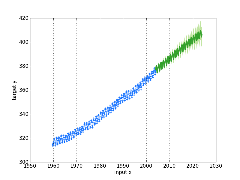
and the optimized values of the hyperparameters allow for a principled analysis of different components driving the model.

[1]	Keeling, C. D. and Whorf, T. P. (2004). Atmospheric $CO_2$ Records from Sites in the SIO Air Sampling Network. In Trends: A Compendium of Data on Global Change. Carbon Dioxide Information Analysis Center, Oak Ridge National Laboratory, Oak Ridge, Tenn., U.S.A.

Regression on Mauna Loa data¶

Table Of Contents

This Page

Navigation

Regression on Mauna Loa data¶

Table Of Contents

This Page

Quick search

Navigation