Basic Regression

The code shown in this tutorial can be executed by running pyGPs/Demo/demo_GPR.py

This demo will not only introduce the regression model, it also provides the general insight of how to use the package. This general information will not be repeated in the other demos.

Import packages

Once you installed pyGPs, the typical way to import it is:

import pyGPs
import numpy as np

Load data

First, load the data for this demo. The data consists of 1-d data points drawn from a unit Gaussian. This is the same data used in the GPML example (it is hardcoded in data/regression_data.npz).

Note that target vector can be in 2d matrix with shape (nn,1) or 1d vector with shape (nn,) where is number of test inputs. pyGPs can work with either format.

demoData = np.load('regression_data.npz')
x = demoData['x']      # training data
y = demoData['y']      # training target
z = demoData['xstar']  # test data

A five-line toy example

Now lets do regression with Gaussian processes. Using pyGPs for regression is really simple; here is the most basic example:

model = pyGPs.GPR()      # specify model (GP regression)
model.getPosterior(x, y) # fit default model (mean zero & rbf kernel) with data
model.optimize(x, y)     # optimize hyperparamters (default optimizer: single run minimize)
model.predict(z)         # predict test cases
model.plot()             # and plot result

By default, GPR uses a zero mean, the rbf kernel and a Gaussian likelihood. Default optimizer is a single run of Rasmussen’s minimize. You will see below how to set non-default values in another example.

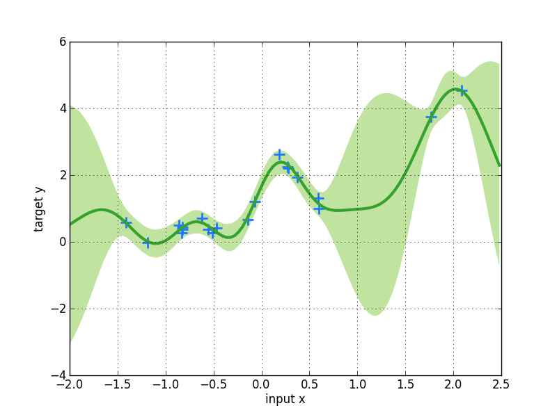
pyGPs.GPR().plot() will plot the result, where the dark line is the posterior mean and the green-shaded area is the posterior variance. Note, that plot() is not a general method as it is not trivial to visualize high dimensional data. Here, pyGPs.GPR().plot() works for 1-d data only, while pyGPs.GPC().plot() is a toy method visualising 2-d input data in a classification scenario.

A more complicated example

Now lets do another example to get insight into more advanced features of the toolbox.

You can specify non-default mean and covariance functions:

m = pyGPs.mean.Linear( D=x.shape[1] ) + pyGPs.mean.Const()
k = pyGPs.cov.RBF()
model.setPrior(mean=m, kernel=k)

Here, we use a composite mean as the sum of a linear and a constant function, and an rbf kernel. The initial hyperparameters are left to their default values. See Kernels & Means for a complete documentation of kernel/mean specification and custom kernel/mean construction. Once kernel and mean are specified, they are passed to the prior using setPrior().

You can add the traning data to the model explicitly by using setData(). So, you avoid passing them into getPosterior() or optimize() each time used. More importantly, the deafult mean will be adapted to the average value of the trainging labels (if you do not specify mean function by your own).

Further, you can plot the data in the 1-d case:

model.plotData_1d()

You can specify a optimization method different from the default, which is a single run of Rasmussen’s minimize. For example, you can choose to rerun the optimization method several times with different random initializations:

model.setOptimizer("Minimize", num_restarts=30)

The optimized hyperparameters returned by optimize() are then set to be the ones obtained from the run with the best result. The whole functionality for optimization is introduced in detail in the documentation Optimizers.

Instead of getPosterior(), which only fits data using given hyperparameters, optimize() will optimize hyperparamters based on marginal likelihood:

model.optimize()

There are several properties you can get from the model:

model.nlZ                   # negative log marginal likelihood
model.dnlZ.cov              # direvatives of negative log marginal likelihood
model.dnlZ.lik
model.dnlZ.mean
model.posterior.sW          # posterior structure
model.posterior.alpha
model.posterior.L
model.covfunc.hyp
model.meanfunc.hyp
model.likfunc.hyp
model.fm                    # latent mean
model.fs2                   # latent variance
model.ym                    # predictive mean
model.ys2                   # predictive variance
model.lp                    # log predictive probability

For example, to get the log marginal likelihood use:

print 'Optimized negative log marginal likelihood:', round(model.nlZ,3)

Prediction on the test data will return five values, which are output mean (ymu) resp. variance (ys2), latent mean (fmu) resp. variance (fs2), and log predictive probabilities (lp)

ym, ys2, fm, fs2, lp = model.predict(z)

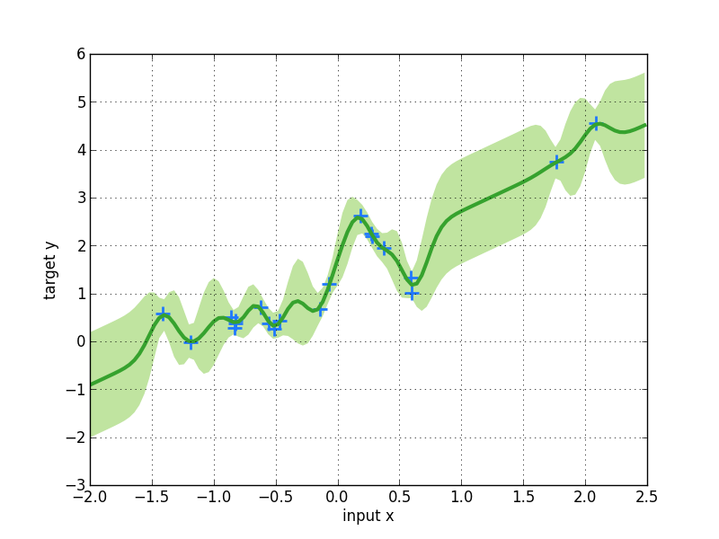
Plot data. Note that GPR.plot() is a toy method only for visualising 1-d data. Here we got a different posterior by using a different prior other than in the default example.

model.plot()

A bit more things you can do

[For all Models] Speed up computation time for prediction if you know posterior in advance. Posterior is passed as an object with three fields (attributes) post.alpha, post.sW and post.L. How to use these vectors to represent the posterior can be best seen from Algorithm 2.1 (page 19) in Chapeter 2 of the GPML book by Rasmussen and Williams, 2006.

post = myPosterior()        # known in advance
ym, ys2, fm, fs2, lp = model.predict_with_posterior( post,z )

[Only for Regression] Specify noise of data (with by default):

model.setNoise( log_sigma = np.log(0.1) )

You do not need to specify the noise parameter if you are optimizing the hyperparamters later anyhow.

All plotting methods have keyword axisvals. You can adjust plotting range if you want. For example:

model.plot(axisvals = [-1.9, 1.9, -0.9, 3.9])

Switch to other Inference and Likelihood functions.

model.useInference("EP")
model.useLikelihood("Laplace")